New methods for the oldest time series of its kind

There are two data attributes which are nearly ubiquitous but often under-appreciated and misunderstood. The first is time: a dimensions which is physically unavoidable, but often ignored to the detriment of predictive power and insight. The second is missing data: a true nuisance for analysis which can also easily become a major pitfall. This is especialy true if, as is often done, overly simplistic methods are relied on and thus major statistical bias introduced.

These ubiquitous and misunderstood attributes have fascinated me on countless projects, but stand forefront on analysis I developed working to unravel climate signals in a multi-decadal environmental series of environmental data. In this project, I looked to analyze how nutrient pollution had changed over decades in Narragansett Bay, across policy changes, and how this had affected the algae (aka phytoplankon) that make the base of the food-web, are responsible for eutrophication, and toxic bloom events.

Though the series is unprecidented in length (>60 years to date), the data has major challenges that require careful design. Missing data is present throughout the series in some cases with durations > 1 year, posing a challenge for unbiased inference. Further the changes to the underlying system, mean we expect the dependence structure evolves through time. Plainly, by this I mean coefficients, covariance, variance, etc. are unlikely to be static along the time dimension, and need to be able to change to describe changing relationships and structure.

Though, I will briefly summarize my work here, you can read my 133 page thesis about it (embedded below)… or read my publication in Statistics and Its Interface, both of which will cover both greater breadth and depth.

Objective:

1. Identify the long-term patterns in key environmental traits & identify the impact of policy change
2. Characterize the seasonal and long-term dependence of algal growth on nutrients
3. Develop a specialized architecture for inference with Bayesian dynamic linear models where missing data imputation is necessary and multiple modeling goals may be required

Data:

The data for this study come from the University of Rhode Island, Long-term Narragansett Bay Monitoring Series (2003-2020). Within this period, from 2005-2012, Rhode Island law mandated a 50% reduction in nutrient pollution from coastal wastewater treatement centers, and a major question as to the efficacy of this action.

Temperature, NH₄ (ammonium), NO₃ + NO₂ (nitrate + nitrite), chlorophyl (chl) <20 μm, chl > 20 μm were the measured features of the series. The chemical variants of nitrogen are known pollutant types to affect algal growth, and the algae itself is measured via it’s dominant pigment (chlorophyl a). The algal measurements are divided on size because of the major effect of size on ecosystem function in everything from food-web interactions to carbon sequestration. Thus, through these measures we hope to see how relevant nutrient polution has changed, and the effect on algae.

Data Processing:

The only processing taken before model development and fit is to perform a natural log transformation on nutrient and chlorophyll levels, simply to reduce skew in the data and meet Gaussian distribution assumptions for model errors. All other attributes with the data (e.g., missingingess, heteroskedasticity in time) I handled with the model architecture.

Analysis and Results

As described above, there are several key applied goals for the environmental series which are made difficult in particular by missing data. Ultimately, the technique I develop is with a multistage model where the first stage serves to analyze univariate time-series traits, and impute missing data with uncertainty, and a second stage is developed to target questions which are multivariate in nature (i.e., how algal biomass is affected seasonally and in the longterm by nutrient pollution).

The General DLM Structure

The core of the modeling approach is the Bayesian dynamic linear model (or DLM), a popular time-series tools which model our data as observations of a latent state evolving through time according to an observation and state equation (eqns. 1, 2). These models have an inherent ability to imput missing data through forward filtering with the Kalman filter followed by backward sampling (Kalman 1960).

Equation 1. Observation equation:

\[Y_t = F_t \Theta_t + v,\quad v \sim N(0,V)\]

Equation 2. State equation:

\[\Theta_t = G_t \Theta_{t-1} + w,\quad w \sim N(0, W)\]

Kalman Filtering and Smoothing:

1. One-step-ahead predictive distribution of the latent state, \(f(\Theta_t \vert y_{1:t-1}) = N(a_t, R_t)\) where:

   \[a_t = E(\Theta_t|y_{1:t-1}) = G_t m_{t-1}\] \[R_t = Var((\Theta_t|y_{1:t-1})) = G_t m_{t-1} G'_t + W_t\]

2. One-step-ahead predictive distribution of the observation, \(f(Y_t \vert y_{1:t-1}) = N(f_t, Q_t)\), where:

   \[f_t = E(Y_t \vert y_{t-1}) = F_t a_t\] \[Q_t = Var(Y_t \vert y_{t-1}) = F_t R_t F'_t + V_t\]

3. The filtered distribution of the latent state, \(f(\Theta_t \vert y_{1:t}) = N(m_t, C_t)\), where:

   \[m_t = E(\Theta_t \vert y_{1:t}) = a_t + R_t F'_t Q^{-1}_t e_t\] \[C_t = Var(\Theta_t \vert y_{1:t}) = R_t - R_t F'_t Q'_t F_t R_t\] \[e_t = Y_t - f_t\]

4. The smoothed distribution of the latent state, \(f(\Theta_t \vert y_{1:T})=N(s_t, S_t)\), where:

   \[s_t = E(\Theta_t \vert y_{1:T}) = m_t + C_t G'_{t+1} R'_{t+1}(s_{t+1} - a_{t+1})\] \[S_t = C_t - C_t G'_{t+1}R^{-1}_{t+1}(R_{t+1})R^{-1}_{t+1}G_{t+1}C_t\]

These models also allow any parameter of our model to time vary, allowing us to study temporally changing relationships. This includes covariance matrices through a method called discount factoring. This method works extremely well for dynamic covariance when data are mostly complete. The method, outlined in West and Harrison 1997, mathematically suggest that the covariance matrix \(W_t\) for the latent state specification of the model, should decay from one time step to the next.

The DLM itself, like a NN or regression is just a general framework to which we can adapt to very specific architecture. Through the general system of equations shown above, very detailed solutions are possible, for example, ARIMAX or dynamic regression are popular architectures. In our case, we build architectures specifically to answer our questions in each of the stages.

Stage 1 Architecture

In stage 1, we setout to answer questions about long-term patterns such as seasonality, and the long-term trend. Thus we can build a structure which specifically includes these components. In the parameterization outlined below, each time-series is modeled with a dynamic intercept (long-term trend, \(\mu\)), and Fourier form seasonal components from a period of 1 year to 23 weeks to capture complex seasonal patterns.

\[F_i^Q = [1,\ (1,\ 0),\ (1,\ 0),\ ...\, (1,\ 0)_J]\] \[G_i^Q = \begin{bmatrix} 1 & \\\ & G_s^Q \end{bmatrix}\] \[G_s^Q = \begin{bmatrix} H_1 & & \\\ & \ddots & \\\ & & H_J \end{bmatrix}\] \[H_j = \begin{bmatrix} cos(\omega_j) & sin(\omega_j)\\\ -sin(\omega_j) & cos(\omega_j) \end{bmatrix}\] \[\omega_j = 2\pi_j/s, j=1, ..., J\] \[\theta_{i,t}^Q = \begin{bmatrix} \mu_i \\\ S_{i,1,t} \\\ S_{*i,1,t} \\\ \vdots \\\ S_{i,J,t} \\\ S_{*i,J,t} \end{bmatrix}\]

Stage 2 Architecture

In the second stage, the goals is to determine the dependence structure between nutrients and algal biomass. Rather than try to model the series entirely with trend and seasonal components, we try to quantify the impact of an exogenous predictor. The second stage model also includes a dynamic intercept, a annual cycle with a period of 1 year, and a dynamic regression component on nitrogen sources. In this way, the model tells us how nitrogen predicts the anomaly from bulk seasonal and long-term patterns which are affected by a plethora of other traits.

\[F_Z = [1, g(X),\ (1,\ 0)]\] \[G_Z = \begin{bmatrix} 1 & & \\\ & 1 & \\\ & & G_s^Z \end{bmatrix}\] \[G_s^Q = H\] \[H_j = \begin{bmatrix} cos(\omega_j) & sin(\omega_j)\\\ -sin(\omega_j) & cos(\omega_j) \end{bmatrix}\] \[\omega_j = 2\pi/s\] \[\theta_{i,t}^Q = \begin{bmatrix} \mu_{i, t} & \dots & \mu_{z,t}\\\ \beta_{1,t} & \dots & \beta_{1,t} \\\ S_{i,t} & \dots & S_{z,t} \\\ S_{*i,t} & \dots & S_{*z,t} \end{bmatrix}\]

Model Fit

The model was fit with Markov-chain monte-carlo to solve for the posterior distribution of each parameter. It’s worth noting that the method of dividing the modeling into two stages allowed the MCMC inference to be carried out independently for each stage. This separation meant that the posteriors from stage 1 could be sampled in stage 2, and the inference on missing data did not need to be repeated in the regression analysis. This added efficiency to the model fitting process.

Results

The study presents a two-stage Dynamic Linear Model (DLM) as a versatile tool for handling noisy, incomplete, and non-monotonic time-series data in long-term environmental monitoring. In this work:

• I successfully applied a new multistage DLM architecture to assess the relationship between phytoplankton populations and dissolved inorganic nitrogen (DIN) levels in the Narragansett Bay.
• The first stage of the model allows characterization of seasonal and long-term change in the data and supports inference into periods of missing data. The completed data series helps in further exploratory analysis.

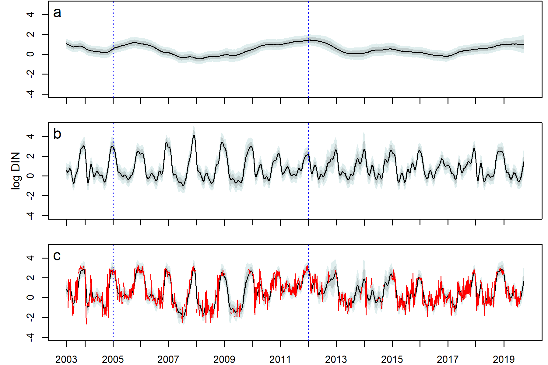
Decomposition of the DIN series DLM (2003–2019), fit with the stage 1 model structure. a. the dynamic intercept, b. the seasonal trend, c. the posterior predicted mean with the true data (red). The median (black), 80% (dark grey shading), and 95% (light grey shading) pointwise credible intervals are shown. Blue dotted lines denote the beginning and end years of policy mandated nutrient remediation.

• The second stage of the model focuses on dynamic regression, working with the latent levels of the predictors, which are devoid of observational uncertainty. This stage examines the dependencies between the studied variables.

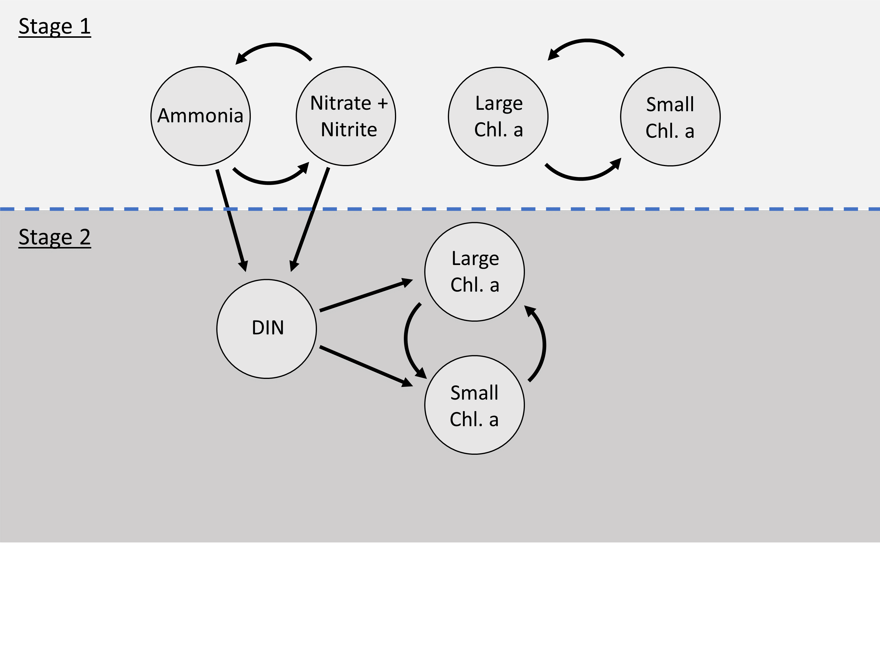
Dependence structure between components of the stage 1 and stage 2 model for the Narragansett Bay ecological model. A bivariate model was run for small and large chl. a as well as nitrate + nitrite to describe long-term patterns among all series. Examination of prewhitened cross-correlations between the imputed series after stage 1 led to the use of DIN as a predictor in stage 2 to explore the influence of nitrogen on size structure of phytoplankton. Stage 2 used latent levels of ammonia and nitrate + nitrite.

• Practical discount methods were found critical for the evolution covariance matrix, preventing over-parameterization and mixing issues in the Markov Chain Monte Carlo (MCMC) algorithm, which is used for estimation and inference in the DLM.

• The multistage DLM allows for the MCMC inference to be carried out independently for each stage, improving computational efficiency by not repeating the inference on missing data in the regression analysis.

• Ultimately, this model answered the key question on how algae blooms were effected by the policy changes. Results suggest that smaller phytoplankton (<20 μm) are relatively unaffected by changes in DIN levels, while larger phytoplankton (>20 μm) show a negative relationship with DIN. This relationship varies seasonally, with the strongest associations occurring in the winter.

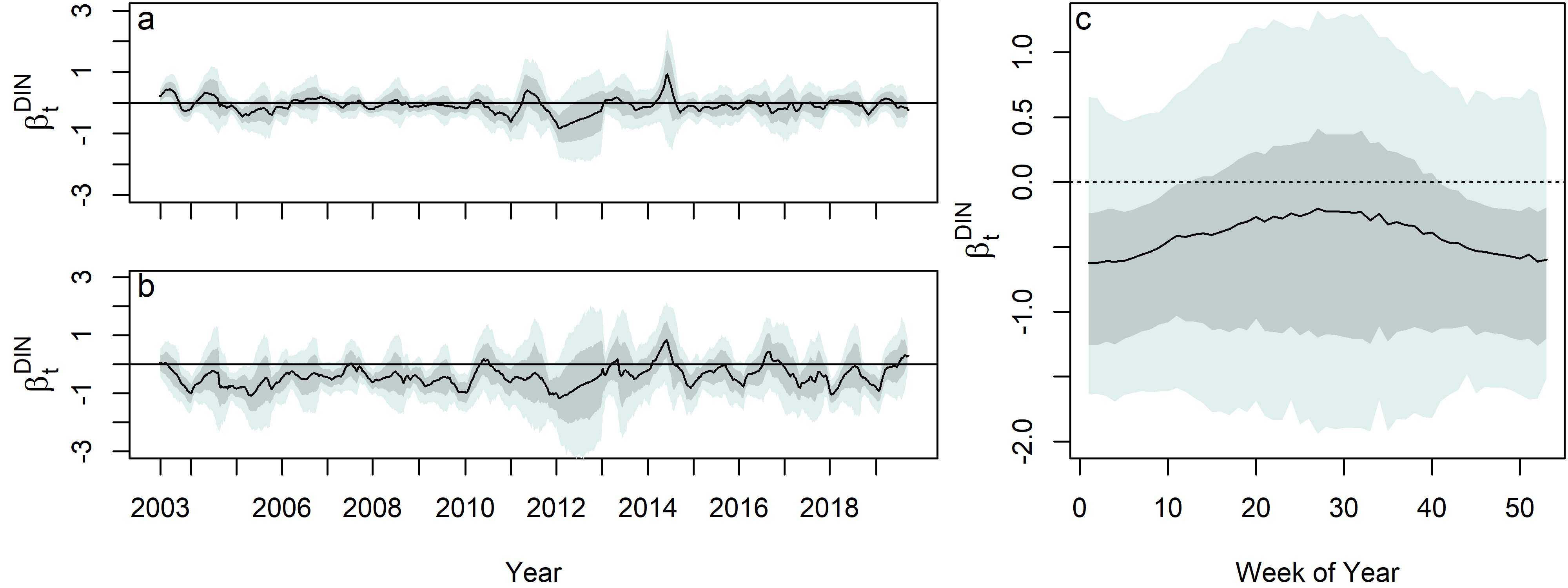
The dynamic regression coefficient, $\beta^{DIN}_t$ , for both the a. Small chl. a series b. Large chl. a series. c. Posterior distribution of the dynamic regression coefficient, $\beta^{DIN}_t$ , on DIN for the large chl. a, plotted by week on the x–axis, and by year as denoted by color shading. The median (black), 80% (dark grey shading), and 95% (light grey shading) are shown.

• The multistage DLM can accommodate data with significant missing points, disparate data streams, and multiple modeling goals.

• The multi-stage state-space model architecture shows value for environmental monitoring and similar long-term analyses.

Conclusions:

• Policy changes did not have a statistically distinguishable effect on Nitrogen levels at the study site (though other research has found localized effects closer to the sources).

• The size of algal organisms shifted from being dominated by large to being dominated by small organisms, which could potentially impact everything from food-web structures to carbon sequestration.

• The dependence on nitrogen has not significantly changed, and is highly seasonal, meaning seasonally targeted efforts, especially in the winter could have the greatest effect on algal growth.

• Practical discounting methods, though previously untested, show superior accuracy for imputation in cases of non-static covariance.

• The multi-stage architecture is particularly advantageous for modeling efforts with multiple goals and extensive missing data. With this architecture, the first stage can server to both characterize the time-series and provide advanced multiple imputation, leaving the flexibility to experiment in the second stage with a more parsimonious model.