Mathematical models of microbial growth

Marine microbes are some of the most numerous organisms in the world. Although you may have never seen or though about them, they make our planet survivable in many ways (not the least of which is producing 50% of the atmospheric oxygen we breathe and forming the base of the food we in all the world’s oceans). Despite being so numerous and critical to life on our planet, there are major gaps in our understanding of how these tiny organisms are shaped by their environment.

Under a fellowship with NASA Space Grant, I studied how temperature impacts these critical organisms. In this project, by creating mathematical models of microbial growth and size as a function of temperatures, I provided a small piece of NASA’s large numerical models that work to model and predict our own planetary function.

If you would like the full details of the published study, you can read it here:

Objective:

Measure the growth and cellular size traits of a globally relevant marine algae.

Mathematically model how the cellular traits are impacted by temperature. Use interpretable statistical models that can be used for prediction and ecological interpretation. From the start, we had several targeted questions:

1. How do populations of microbes grow across a wide range in temperatures?
2. How are the sizes of the microbial cells impacted across a wide range in temperature?
3. How much do changes in temperature (thermal perturbations) impact population growth?
   • Does the impact from change itself impact our ability to estimate temperature effects?

Use ocean thermal data and mathematical models of thermal responses to estimate the magnitude of thermal effects on microbial function.

Data:

Cells and Culture Growth

As a study case for the biological response of algae to temperature and temperature change, I chose an algae which is both common and toxic, Heterosigma akashiwo. The cells were kept healthy, in exponential growth. To avoid convolution of the thermal response with the response to new media, cultures were only transferred to new media more than 1 d prior to and 1 d post to a change in temperature.

Temperature treatments

With little prior information as to which features of changing temperature might influence growth, two major traits were examined in the experimental design: (1) the direction of temperature change (increasing or decreasing) and (2) the magnitude of temperature change (small shifts vs. larger cumulative changes). To address these features, and represent realistic rates of change, cultures were shifted sequentially to new growth temperatures outward from 15\(^{\circ}\)C (Fig. 1). Including the control culture, growth rate, and acclimation was measured at 10 temperatures: 6\(^{\circ}\)C, 8\(^{\circ}\)C, 10\(^{\circ}\)C, 12\(^{\circ}\)C, 15\(^{\circ}\)C, 18\(^{\circ}\)C, 22\(^{\circ}\)C, 25\(^{\circ}\)C, 28\(^{\circ}\)C, and 31\(^{\circ}\)C. As each incubator had a static temperature, we used small discrete shifts in temperature over time. Beginning with the culture that was acclimated to 15\(^{\circ}\)C, every 4 d a triplicate set of the cultures growing at the highest and lowest current temperatures were split, with one fraction retained at its current temperature and the other fraction shifted one temperature step outward (i.e., further toward the temperature extremes of 6\(^{\circ}\)C and 31\(^{\circ}\)C.

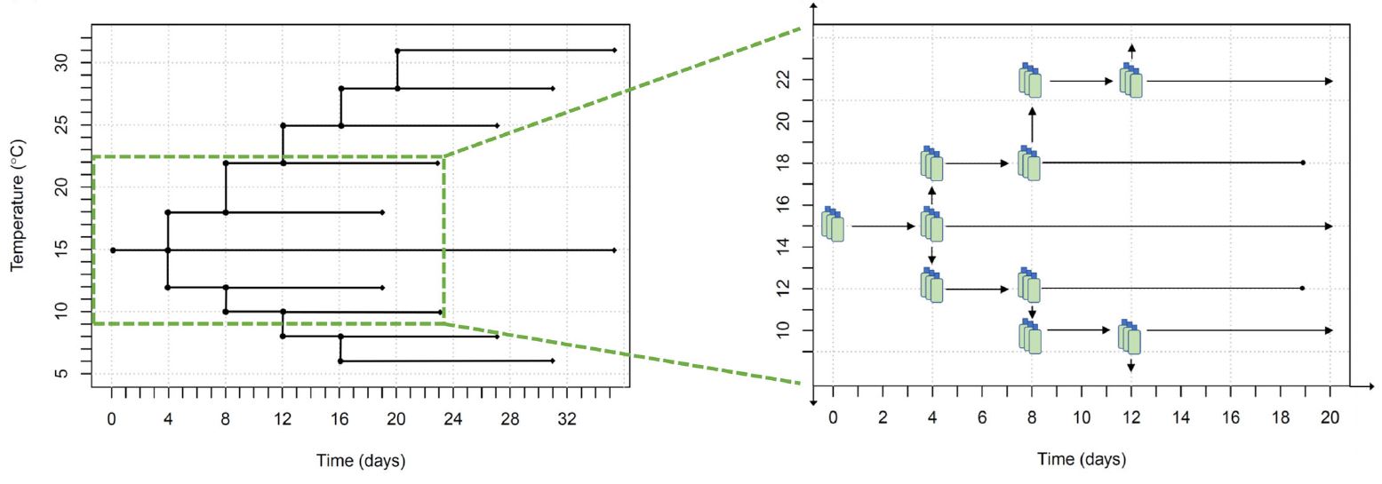Figure 1: Experimental temperature treatement design and temporal component to data collection.

Data Collection

To quantify changes in cell size, population growth rate (cell numbers), and volumetric growth rate, the abundance and cell size distribution were measured with a Beckman Coulter Multisizer 3 for 15 d following the initial transfer to the target temperature.

Data Processing:

The measurement taken in this study, for which, all statistics are derived are cell size distributions. The Coulter counter is a machine which counts the number of particles in size bins from ~1 to 100 \(\mu\)m. Measuring the number of cells in culture with automated instruments, can be produce suprisingly noisy data that need to be cleaned. Particularly, decaying material and undesireable cell populations in the culture may show signals in the data.

While normally the data are processed by hand, I automated the processing of thousands of cell distributions by fitting a mixture of a Gaussian and exponential mixuture model to the cell size distribution data, I quantified the mean and variance of the size distribution and number of cells in the target population. The traits of these population measures served as the key independent varaibles in the desired mathematical models of growth. Below you can see an example of a cell size distribution with overlaid Gaussian density curves:

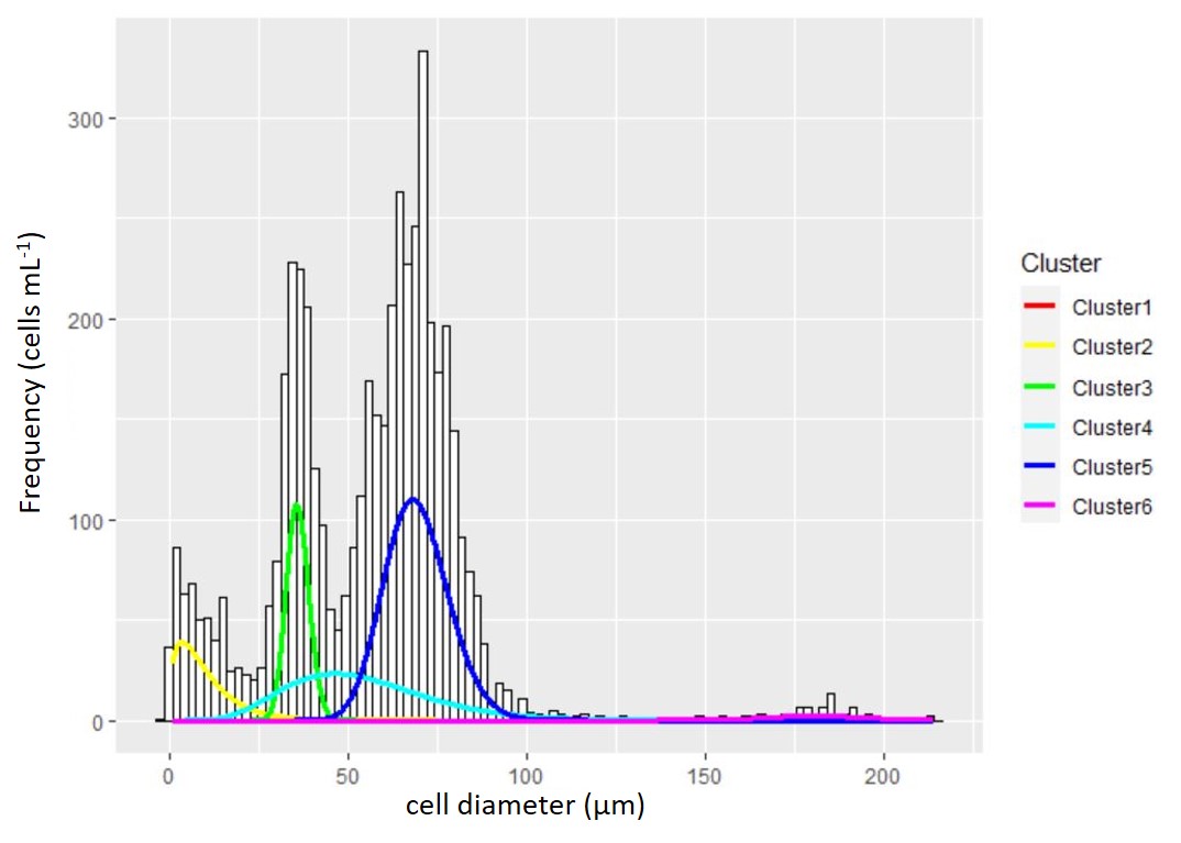Figure 2 : A particle and cell size distribution is fit with a mixture of distributions to identify the true cell count and population characteristics. The raw data collected from the Coulter counter is the underlying histogram of cell size with frequency on the y-axis and cell size on the x-axis. To fit the mixture distribution, the frequency data is first converted to raw measurements of individual cells. The density distributions from the mixture model are overlaid for graphical reference to the model fit. Unlike most clustering cases where the true number of clusters cannot be known, microscopy was used to verify the number of true cell populations and possibly multiple cell size groups of the same population.

Population growth rates were calculated by fitting an exponential growth curve to the population data:

\[P_t = P_0 * e^{rt}\]

where:

• \(P_t\) is the population at time \(t\)
• \(P_0\) is the original population
• \(r\) is the growth rate
• \(t\) is the elapsed time

Analysis & Results:

1.) How does temperature affect growth rate?

With maximum likelihood estimation, I used the calculated specific growth rates were to fit a standard thermal reaction curve used in biology:

\[k(T) = a*e^{bT}[1 - (\frac{T-z}{w/2})^2]\]

where :

• a, b, and z are shape parameters
• w is the thermal niche width
• T is a given temperature
• k(T) is the specific growth rate at that temperature

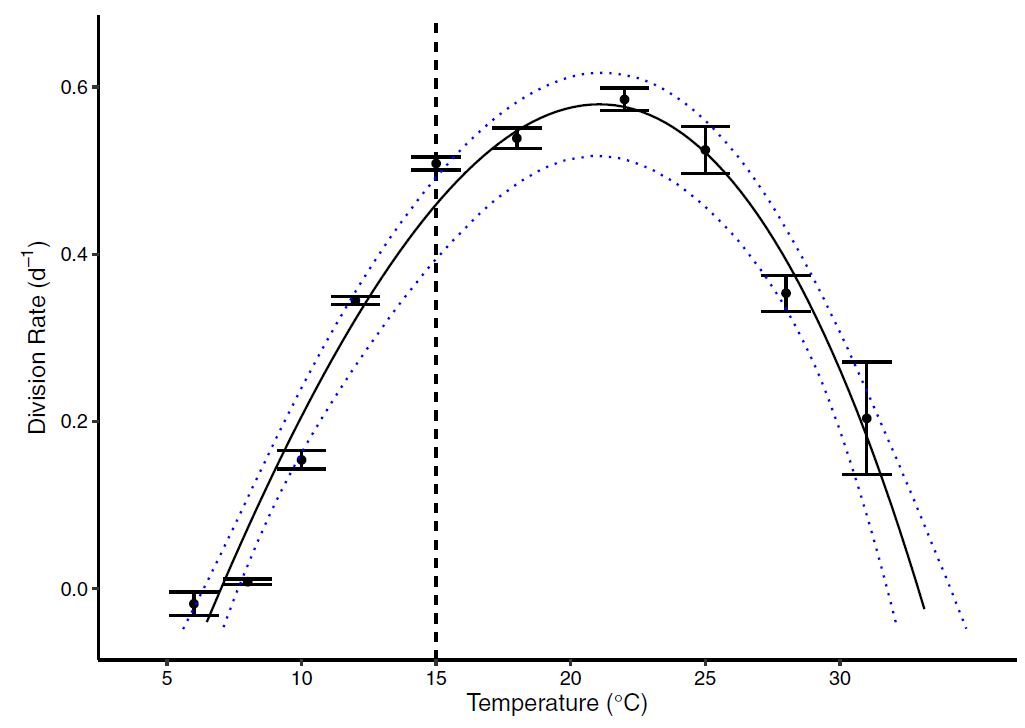Figure 3 : The thermal reaction norm showed a clear thermal dependence with a tolerable range (\(w = 25.9^{\circ}\)) spanning from \(7^{\circ}C\) to \(33^{\circ}\). This upper temperature range suggests that the marine algae can survive to some of the hottest temperatures seen in the ocean, and are likely to tolerate further warming with continued positive growth rates. However, warming beyond the optima (\(z=20^{\circ}C\)) will result in thermal stress.

2.) How are the sizes of cells impacted by temperature?

And analysis of cell size showed that both the devision rate and cell size were closely tied to temperature:

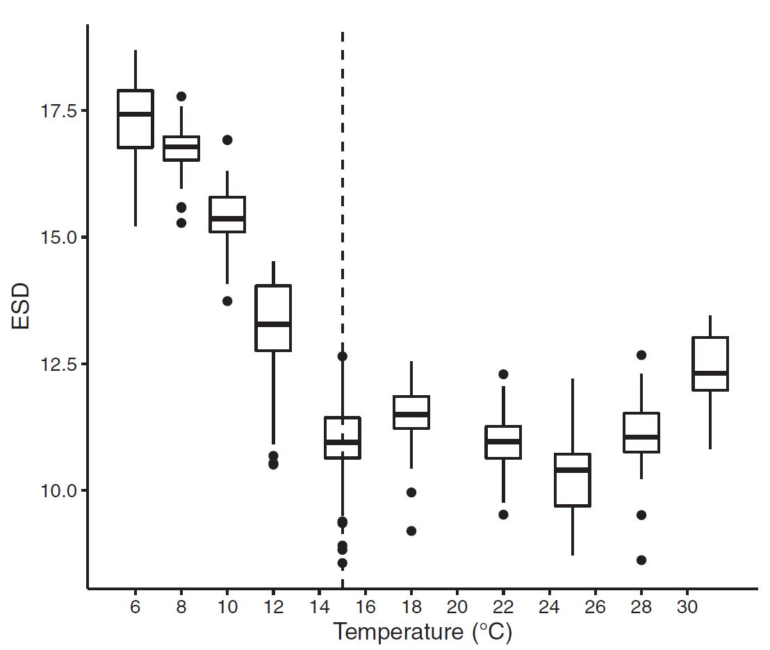Figure 4: ESD (Cell diameter) measurements across temperature. Results show a clear relationship with generally decreasing cell size as temperature increases.

While the relationship between cell size and temperature is strong, nuance here is important. From the graphical outputs, I had noted, the cell size relationships and aberations from linearity seemed to match an inverse of the temperature growth curve. After noting some-nonlinearity in the relationship, and conducting other exploratory comparisons, I tested whether there was another explainatory reason for cell size changes.

After comparing multiple models (AIC) with a type II regression, I showed that cell size was best explained by cell division rates. This is important to our understanding because the evidence suggests that it’s not temperature directly, and potentially any influences on division rates will affect cell size.

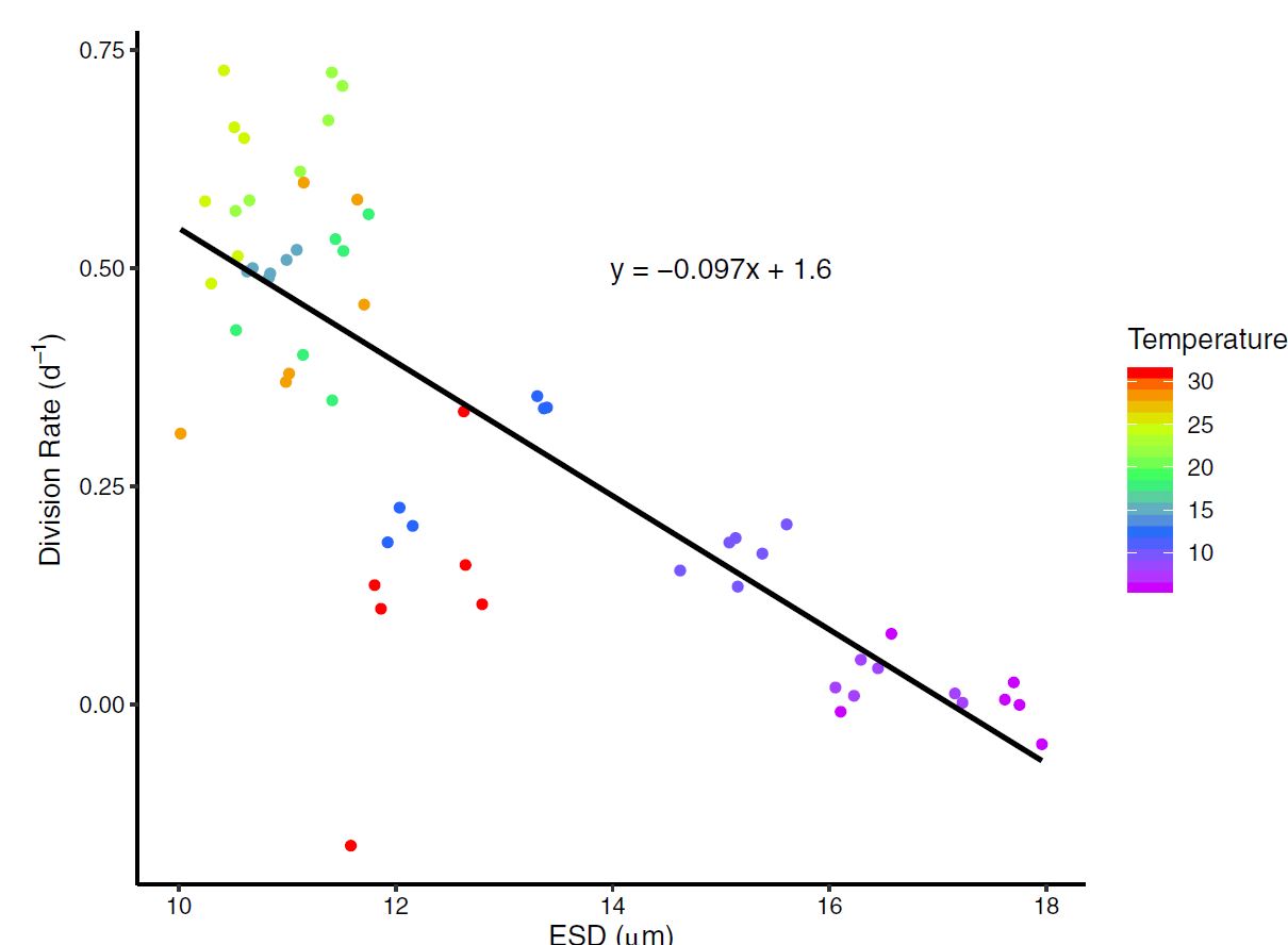Figure 5 : A type II regression fit between ESD (cell size) and division Rate (population growth rate). The temperature treatement where each measurement was recorded is shown in color.

3.) How much does change itself impact population growth and cell size?

To quantify the effect of time (acclimation) on specific growth rate, the final rates (\(\mu_f\), 7 ≤ \(\Delta\) time ≤ 15 d) were subtracted from the initial rates, measured over the first 3 d (\(\mu_0\); \(\Delta\) time ≤ 3 d) for each temperature treatment.

A break-point detection and Dunnet’s test showed three distinct response groups: 1.) Small thermal changes which lowered growth rate immediately 2.) Medium changes which accelerated growth 3.) Extreme changes which again lowered growth. To be brief, there are biological mechanisms we hypothesize which can explain these patterns, but further detailed molecular metabolic research would be needed to understand these response patterns fully. Nonetheless, we have evidence that changing temperature dramatically effects growth rates.

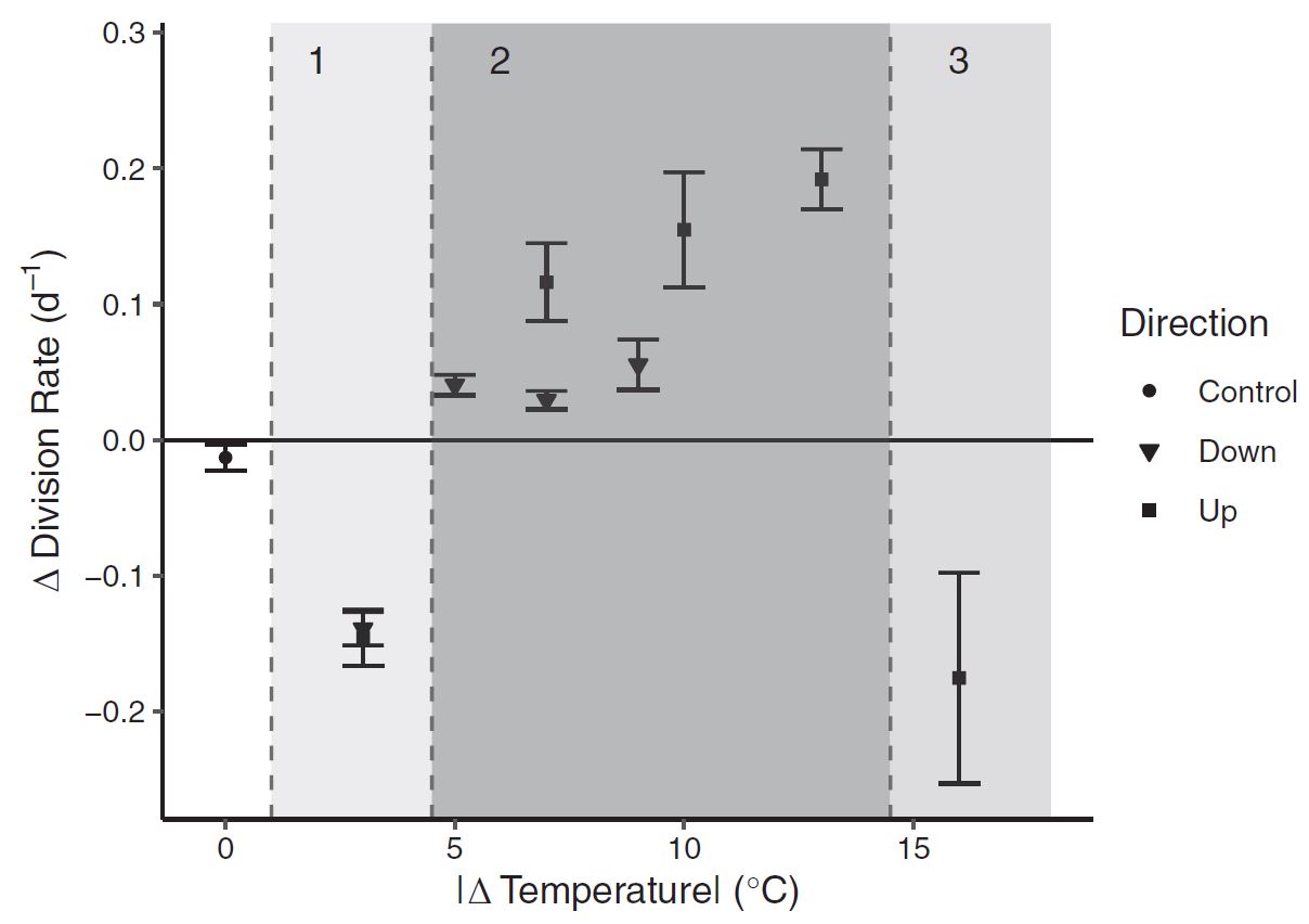Figure 6: Growth rates were dramatically impacted by the cumulative magnitude of temperature change itself.

Last, to understand patterns in the variability of growth rate among replicates as a function of the cumulative temperature change (\(\Delta\)Temperature) and time (translated into a binary variable; \(t_0\) and \(t_f\) to 0 and 1, respectively). After graphically examining the variance in growth rate relative to temperature changes, an exponential relationship was fit to the SD of the specific growth rate (σ). The following regression was again fit with maximum likelihood expectation (MLE):

\[\sigma = c * e^{d*\vert\Delta T\vert - e*time}\]

where:

• c, d, and e are shape coefficients
• \(\sigma\) is the specific growth rate
• T is a given temperature
• t is the time after temperature change

Temperature change caused an exponential level increase in biological variability. And the power of the exponent decreased with time. This may seem esoteric, but the fundamental origins of biolocal variability are an open ended question in biology, and any evidence that can explain why organisms vary is valuable. Here our data evidences how environmental peturbations can rapidly diversify a population.

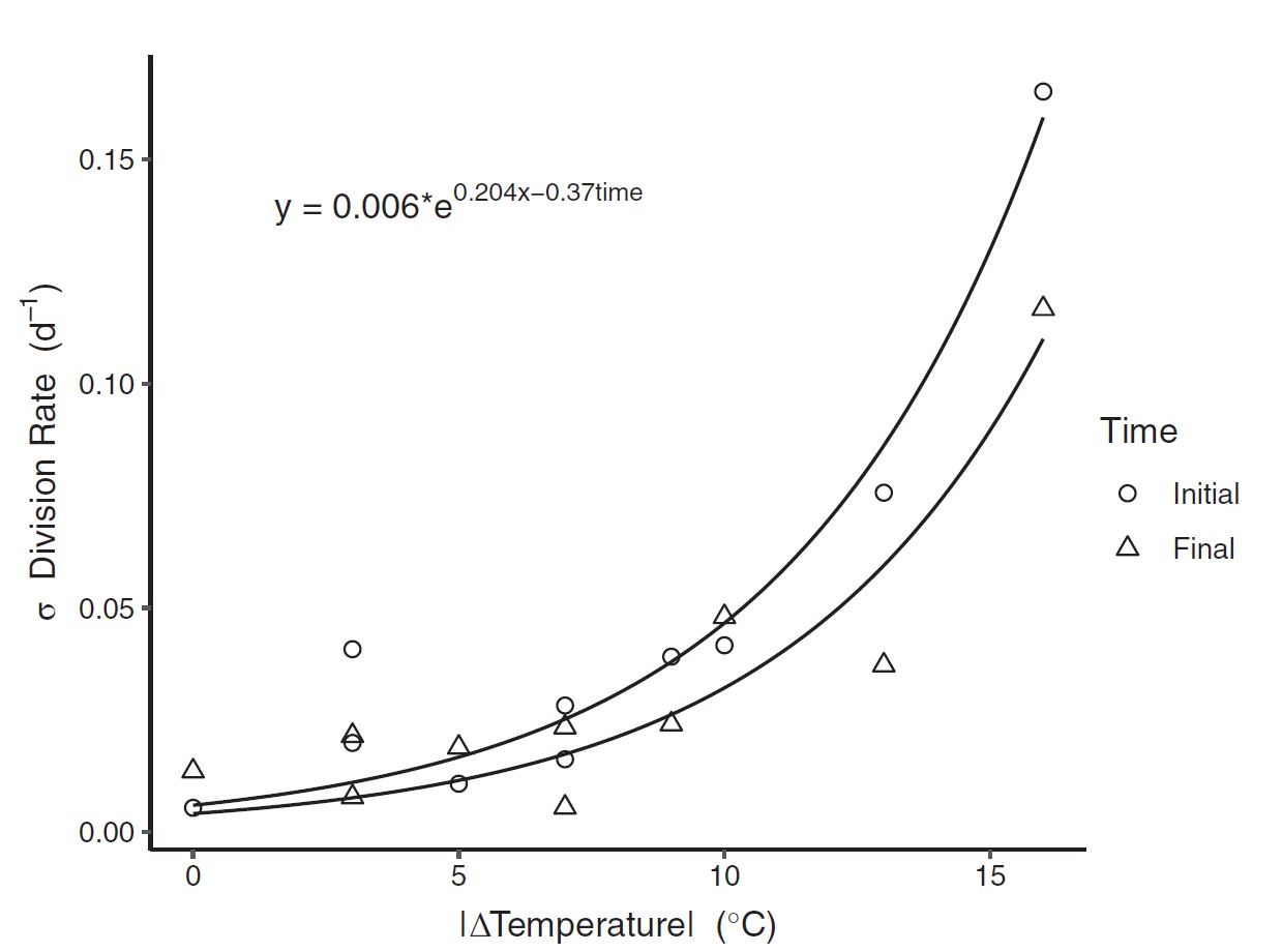Figure 7: Standard deviation in division rate (between replicates) as a function of the magnitude of temperature change. The exponential fit suggests that biological variablity increases exponentially as a result of environmental variation.

How much can thermal variability impact estimates from a standard thermal performance curve?

To exemplify, the impact of the thermal response on microbial growth as well as the potential magnitude of new-found acclimation effects, I extracted seasonal data from varied oceanographic sites within the thermal range of our study organisms. By imputting, this data into the fitted thermal performance curve we made a prediction on population growth and production.

Collecting enough laboratory data to fit any complex function or non-parameteric model to the acclimation data was impossible. As you can see from the raw data of figure 6 above, limited sample size limits the modeling options. Nevertheless, we would be remiss not to make an estimate of potential effects. Using a moving window to quantify the total temperature change an organism would experience, a scaling factor was used based on the response shown in figure 6. Consistent with the results where different magnitudes of temperature change elicited different acclimation responses, we applied a correction equal to the difference in initial and final growth rates observed at each magnitude in temperature change. Specifically, three temperature ranges in the thermal history window elicited different responses: \(3–5^{\circ}C\), \(5–13^{\circ}C\), or greater than \(13^{\circ}C\) (see “Results” section). The average specific growth rate difference (i.e., acclimation) for these three thermal ranges were −0.14 \(d^{−1}\), 0.10 \(d^{−1}\), and −0.18 \(d^{−1}\), respectively. These differences were added to the acclimated rate interpolated from the thermal performance curve. That is, when the thermal history window had a temperature range of \(3–5^{\circ}C\), \(5–13^{\circ}C\), or greater than \(13^{\circ}C\), a −0.14, 0.10, or −0.18 \(d^{−1}\) correction was added to the growth rate inferred from the thermal performance curve. Cases where no growth was observed wereomitted. The percent difference between final and initial growth responses were compared for each day.

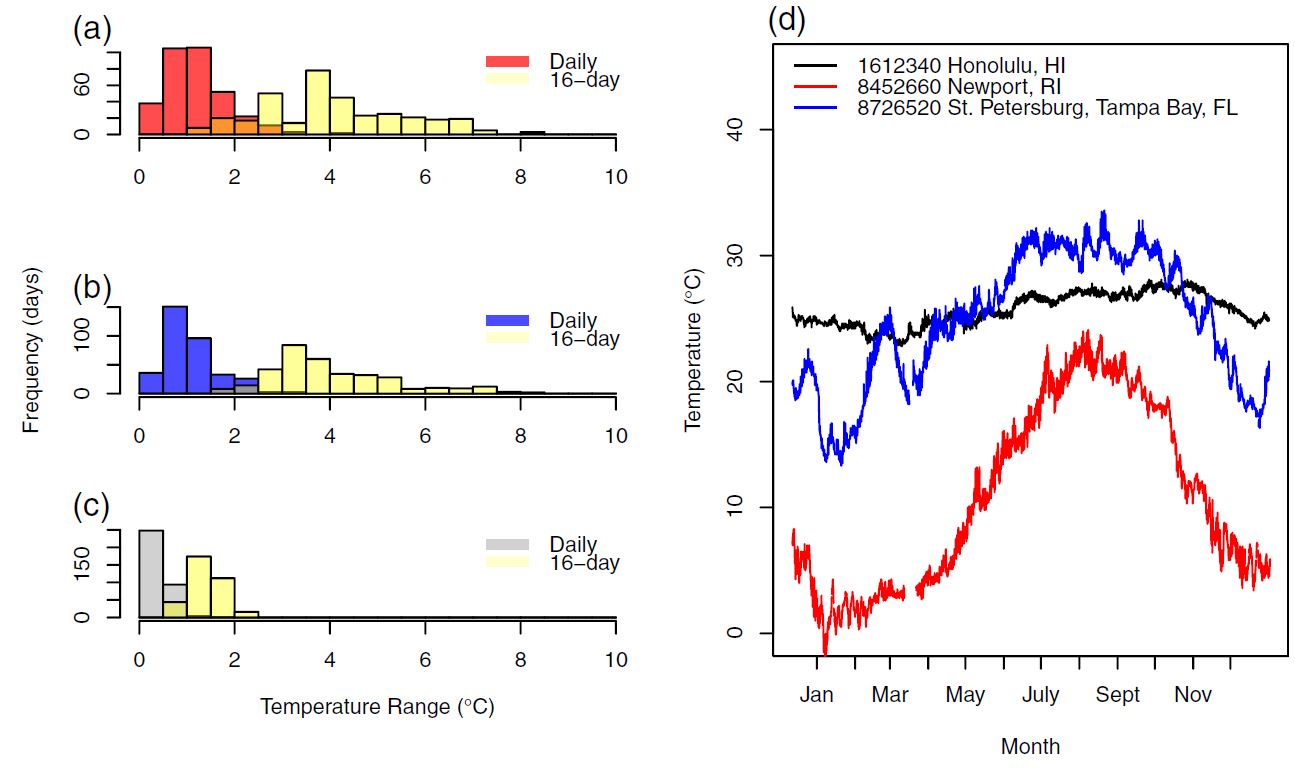Figure 7: With real-world data used for simulation, within the habitat of our target organism, temperature frequently varied to levels where we had seen measureable response to the variability itself.

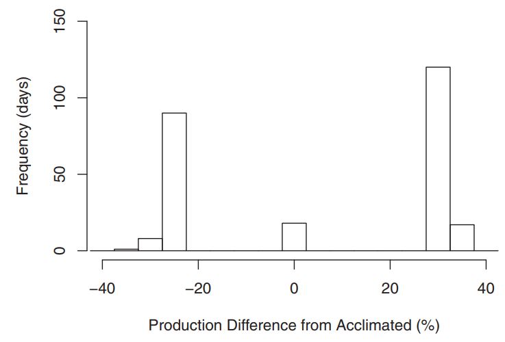Figure 8: Comparing cases to when acclimation was and wasn’t accounted for, there was potential for major discrepencies in growth estimates. The x-axis shows the magnitude of population growth differences in percent. The y-axis shows the number of days (out of 1 year) falling in each histogram bin. This results suggest that in any environment with high seasonality, further research to quantify variabilty responses will be necessary for accurate estimations.

Conclusions:

• Marine algae are highly dependent both on the magnitude of temperature, as well as thermal fluctuations
• Cell size of microbial organisms carry a clear linear relationship to division rate, and consequently may appear to vary with temperature.
• This toxic algae can handle a wide range in temperatures, and in many habitats may see continued increase in growth as the planet warms
• Biological variability intensifies exponentially as the environment changes (as seen through thermal shifts)
• Acclimation responses can impact estimates of biological production 36% under ordinary seasonal thermal conditions.