An improved method for missing data in time series

Time series analysis is the topic that has gripped me since I started studying statistics. Who doesn’t want to better understand the past and predict the future? Most of the data that is collected has a time component which is non-negligable. While some consider the non-independence of data a nuissance for statistical analysis, I consider it one of the greatest opportunities to understand the time pattern.

Time series analysis and time series of data are powerful for building our understand on a topic, but there is almost invariably a big challenge: missing data. Measuring devices brake, data collection is interupted, and periodically the funding may dry up. The way that we handle this missing data can have large effects and potential biases for our inference.

Bayesian state-space models and the particular case of the dynamic linear model are popular time-series tools which model our data as observations of a latent state evolving through time according to an observation and state equation (eqns. 1, 2). These models have an inherent ability to imput missing data through forward filtering with the Kalman filter followed by backward sampling (Kalman 1960).

Equation 1. Observation equation:

\[Y_t = F_t \Theta_t + v,\quad v \sim N(0,V)\]

Equation 2. State equation:

\[\Theta_t = G_t \Theta_{t-1} + w,\quad w \sim N(0, W)\]

Kalman Filtering and Smoothing:

1. One-step-ahead predictive distribution of the latent state, \(f(\Theta_t \vert y_{1:t-1}) = N(a_t, R_t)\) where:

   \[a_t = E(\Theta_t|y_{1:t-1}) = G_t m_{t-1}\] \[R_t = Var((\Theta_t|y_{1:t-1})) = G_t m_{t-1} G'_t + W_t\]

2. One-step-ahead predictive distribution of the observation, \(f(Y_t \vert y_{1:t-1}) = N(f_t, Q_t)\), where:

   \[f_t = E(Y_t \vert y_{t-1}) = F_t a_t\] \[Q_t = Var(Y_t \vert y_{t-1}) = F_t R_t F'_t + V_t\]

3. The filtered distribution of the latent state, \(f(\Theta_t \vert y_{1:t}) = N(m_t, C_t)\), where:

   \[m_t = E(\Theta_t \vert y_{1:t}) = a_t + R_t F'_t Q^{-1}_t e_t\] \[C_t = Var(\Theta_t \vert y_{1:t}) = R_t - R_t F'_t Q'_t F_t R_t\] \[e_t = Y_t - f_t\]

4. The smoothed distribution of the latent state, \(f(\Theta_t \vert y_{1:T})=N(s_t, S_t)\), where:

   \[s_t = E(\Theta_t \vert y_{1:T}) = m_t + C_t G'_{t+1} R'_{t+1}(s_{t+1} - a_{t+1})\] \[S_t = C_t - C_t G'_{t+1}R^{-1}_{t+1}(R_{t+1})R^{-1}_{t+1}G_{t+1}C_t\]

These models also allow any parameter of our model to time vary, allow us to study temporally changing relationships. This includes covariance matrices through a method called discount factoring. This method works extremely well for dynamic covariance when data are mostly complete. The method, outlined in West and Harrison 1997, mathematically suggest that the covariance matrix \(W_t\) for the latent state specification of the model, should decay from one time step to the next.

Discounting Covariance:

\[R_t = Var(\Theta_t \vert y_{1:t-1}) = G_t C_{t-1} G'_t + W_t\] \[R_t = P_t + W_t\] \[W_t = \frac{1-\delta}{\delta}P_t\]

Practically, this equation represents how the information is lost from one time step to the next.

The issue is that for data with extended periods of missingness, standard discounting methods would have the loss of information grow at an exponential rate in the forward filter. If we are predicting \(k\) steps ahead with data, then the covariance at step \(k\) ahead becomes:

\[C_t(k) = \frac{G^k C_t G'^{k}}{\delta^k}\]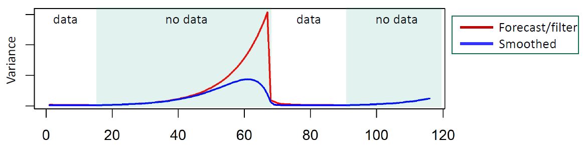

This is as opposed to a linear rate in a static covariance specification that comes with the Kalman filter above:

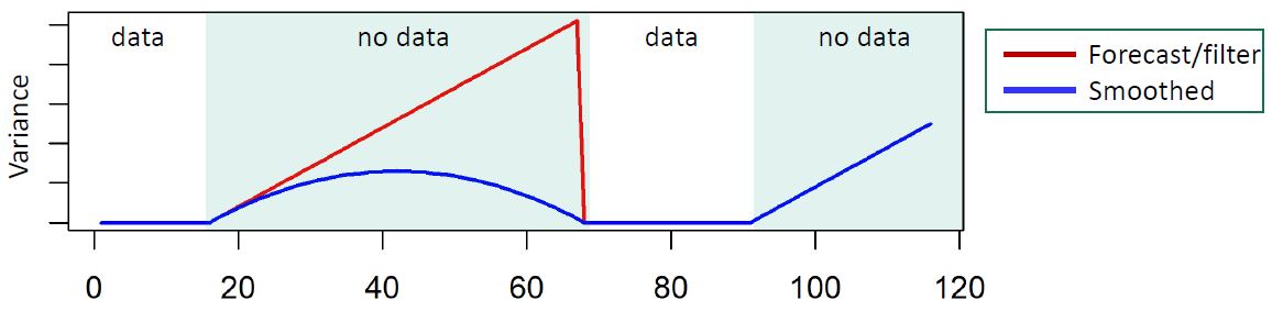
Inutition suggests that an exponential loss of information in missing data may be overly conservative, but what covariance specification gives us the most accurate results for periods of extensive missing data?

Further, what is the optimal selection criteria for selecting a discount factor?

Objectives:

1. Identify the optimal discounting strategy for prolonged periods of missingness

2. Identify the criteria with the strongest statistical power to compare models with different configurations such as fixed discount factors.

Data :

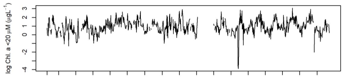
This theoretical investigation was spurred by real time series data from the Narragansett Bay Long-term Time Series. I will use the log transformed Chlorophyll (algal pigment data), because it is the subject of another time series analysis I have been working on. The data is from 2003 to 2020, collected at weekly resolution. While the use of a multivariate analysis would be optimal for imputation, I use a univariate series to focus on the question of covariance specification.

Raw data can be found here.

Data Processing:

While it might seem counter-intuitive, I am using the real data from the time-series to parameterize known data generation models. I choose to do this over completely random data generation models becuase this theoretical investigation is directly tied to the applied problem of analyzing the real data with heteroskedastic behavior and prolonged missingness.

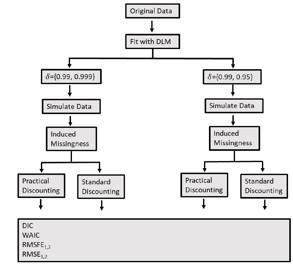
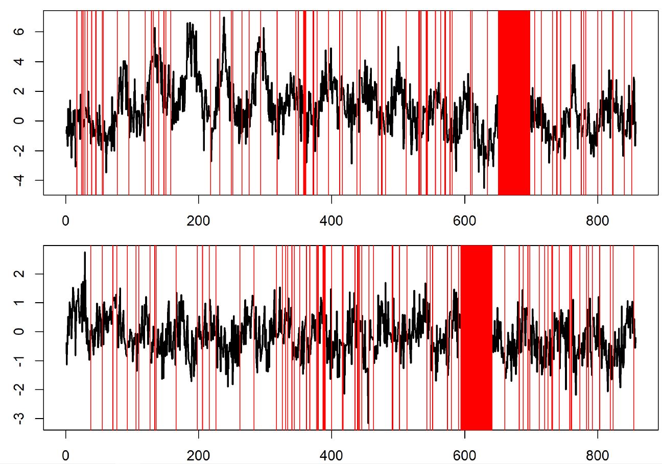
The data were first logged transformed due to their highly positively skewed nature. Second, a dynamic linear model was fit to the data. To capture long-term trend and seasonal behavior, the latent state contained a dynamic intercept and fourier form seasonal components. The models were fit with different levels of fixed discount factors. The posteior mean of \(V\) and \(W_t\) was calculated. New data series were generated from each model fit, with known parameterization. In each copy of the simulated series, missingness was randomly introduced with a frequency distribution matching the original data.

Analysis & Results:

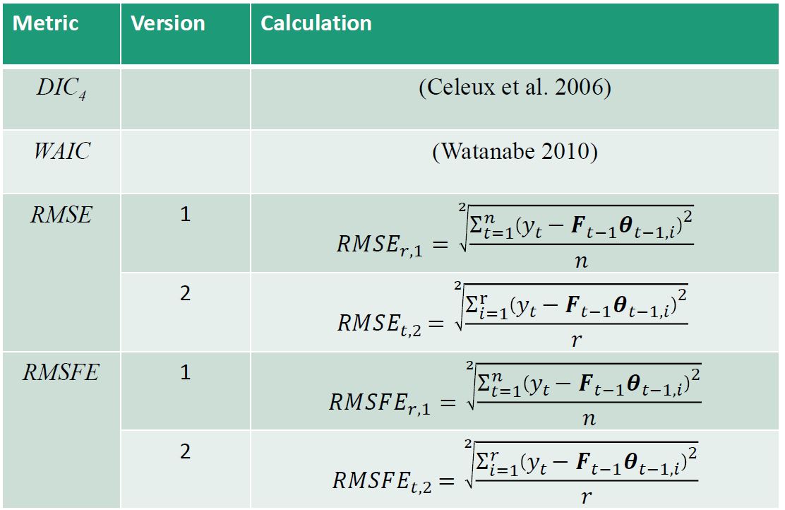
With the simulated data, DLMs were fit with different discount factor levels. The idea is to see if we can recover the discount factors of the data generation model, and which performance criteria helps us make this recovery with the highest accuracy and statistical power. Six performance metrics were calculated and compared to identify which most strongly identified the correct data generation structure.

Performance metrics were compared between fits with practical and standard discounting.

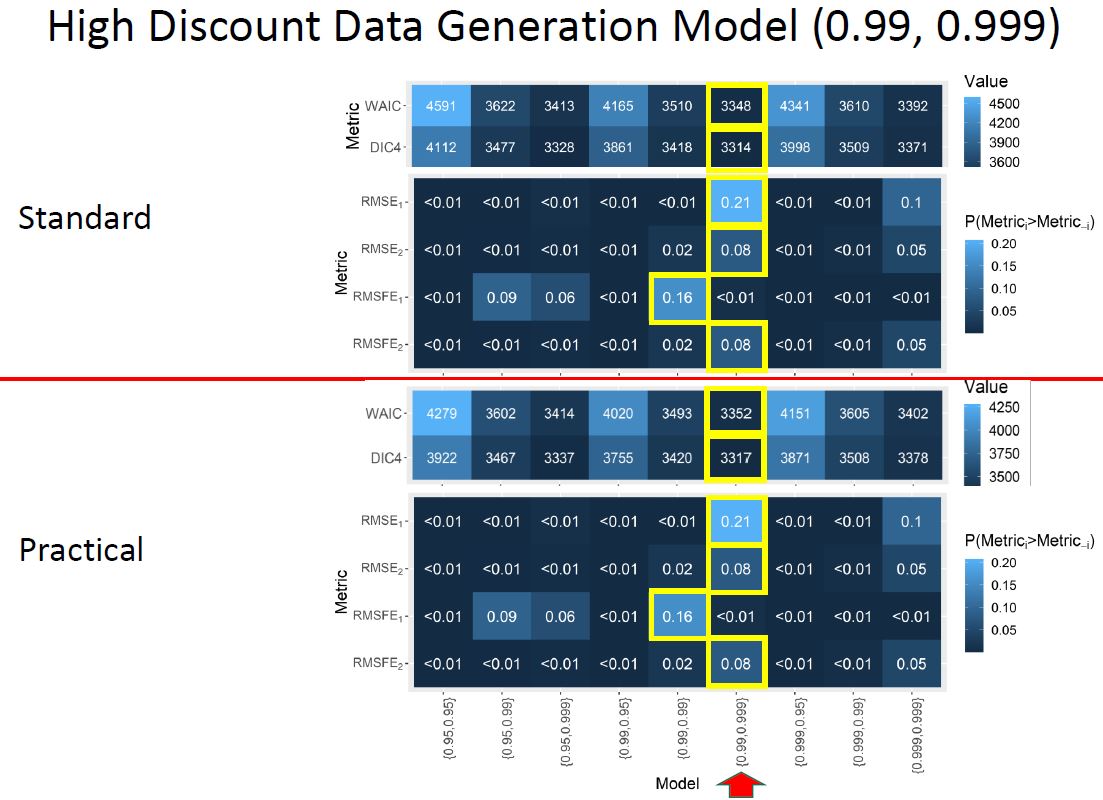
For the data generation model of high discount factors our performance metrics are the following for each model fit, where the x-axis is a set of discount factors used in a model fit:

For the data generation model of low discount factors our performance metrics are the following for each model fit, where the x-axis is a set of discount factors used in a model fit:

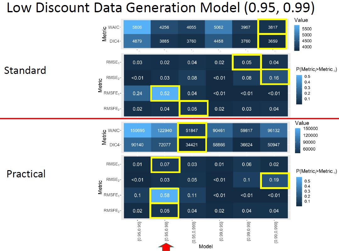
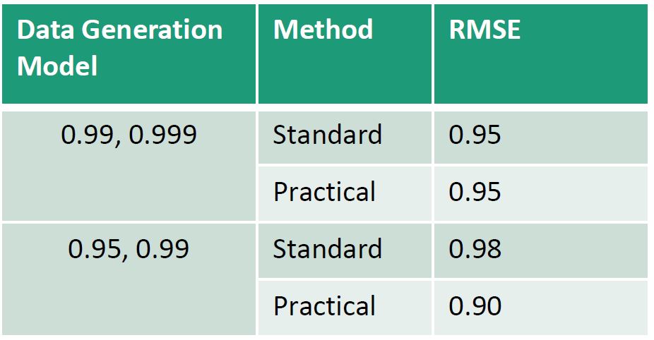
Comparing the standard and practical discounting methods we find the following for each data generation model:

Conclusions:

• Under data simulated with a pair of high discount factors (0.999, 0.99), all metrics selected within 0.009 of the parameters for data generation
• Consistently, $RMSFE_1$ had the most statistical power to recover the parameterization of the data generation model.
• $RMSE$ suggests practical discounting will optimize performance in long-periods of missingness
• DIC support practical discounting imporves the model fit within sample
• Although $RMSE$ was a biased metric for model selection, particularly during prolonged periods of missingness, it still had utility in evaluating the performance of practical discounting in data with long period missingness.
• While $RMSFE$ may be the optimal method for discount factor selection, it does not account for performance during longperiod missingness as our metric of RMSE does. Therefore, results of RMSE in comparable models with practical and standard discounting provide an evaluation for this imputation method.

Literature Cited:

Kalman, R. E. 1960. “A New Approach to Linear Filtering and Prediction Problems.” Journal of Fluids Engineering, Transactions of the ASME 82 (1): 35 45. https://doi.org/10.1115/1.3662552.

West, Mike, and Jeff Harrison. 1997. Bayesian Forecasting and Dynamic Models . 2nd ed. Verlag New York: Springer. https://doi.org/10.1007/b98971.