Predicting Urgent Care Demand Under Uncertainty

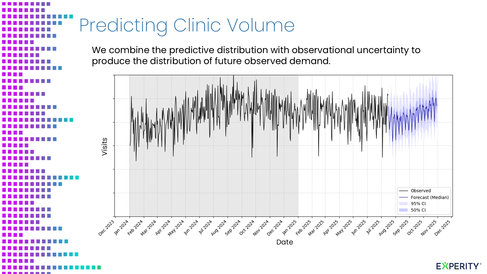
Staffing plans across 45 urgent care clinics had to be made before demand was known. The apparent modeling question was: How many patients will visit each clinic on a given day?

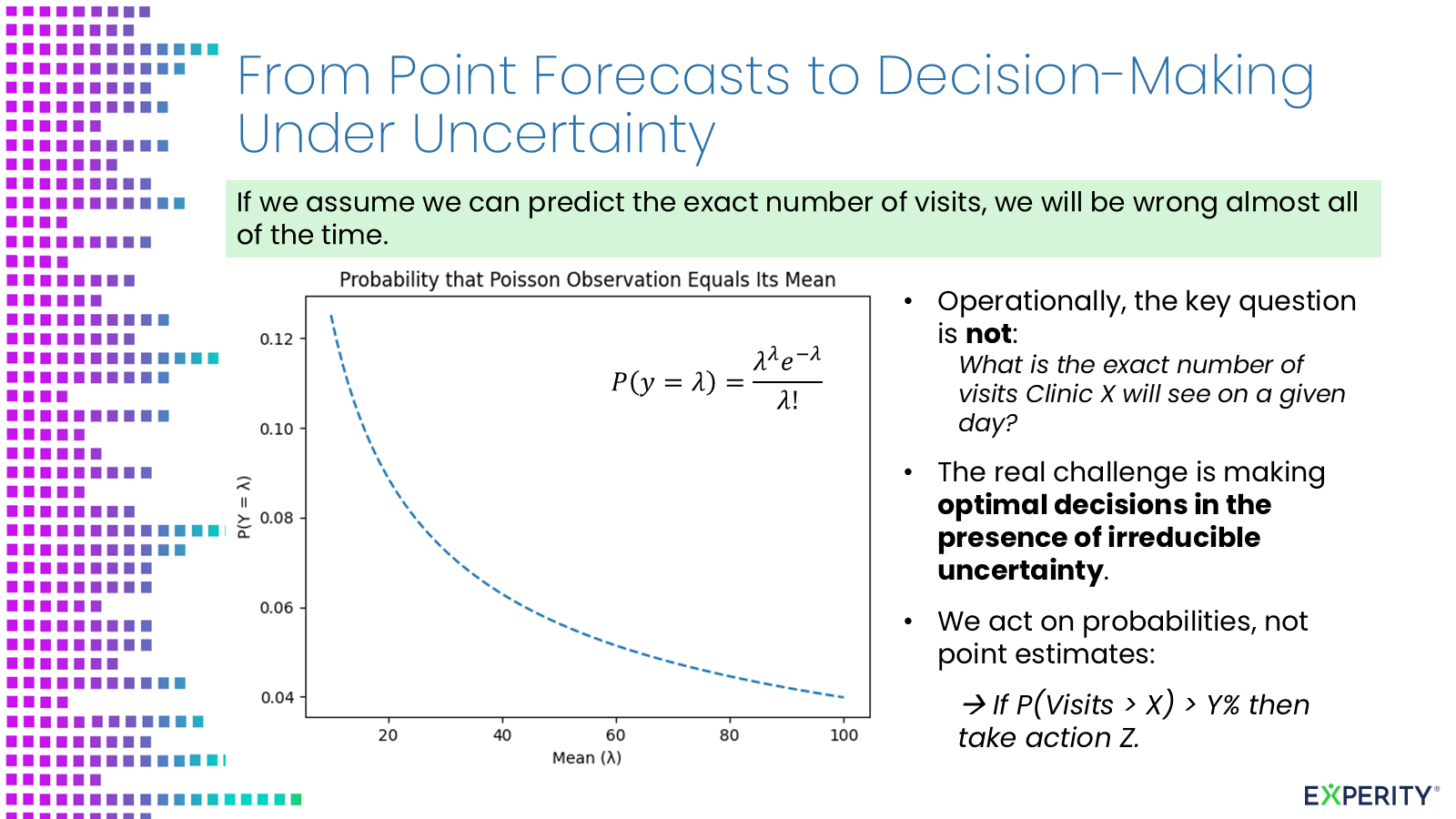
That question invites a point forecast—perhaps 42.7 visits—and a familiar search for lower average error. It also misses the decision. A clinic cannot schedule for a fraction of a patient, and two days with the same expected demand can produce different realized volumes.

The useful question was: How likely is demand to exceed the capacity of the planned staff?

That reframing became the central design choice in the forecasting system.

Why a single number is misleading

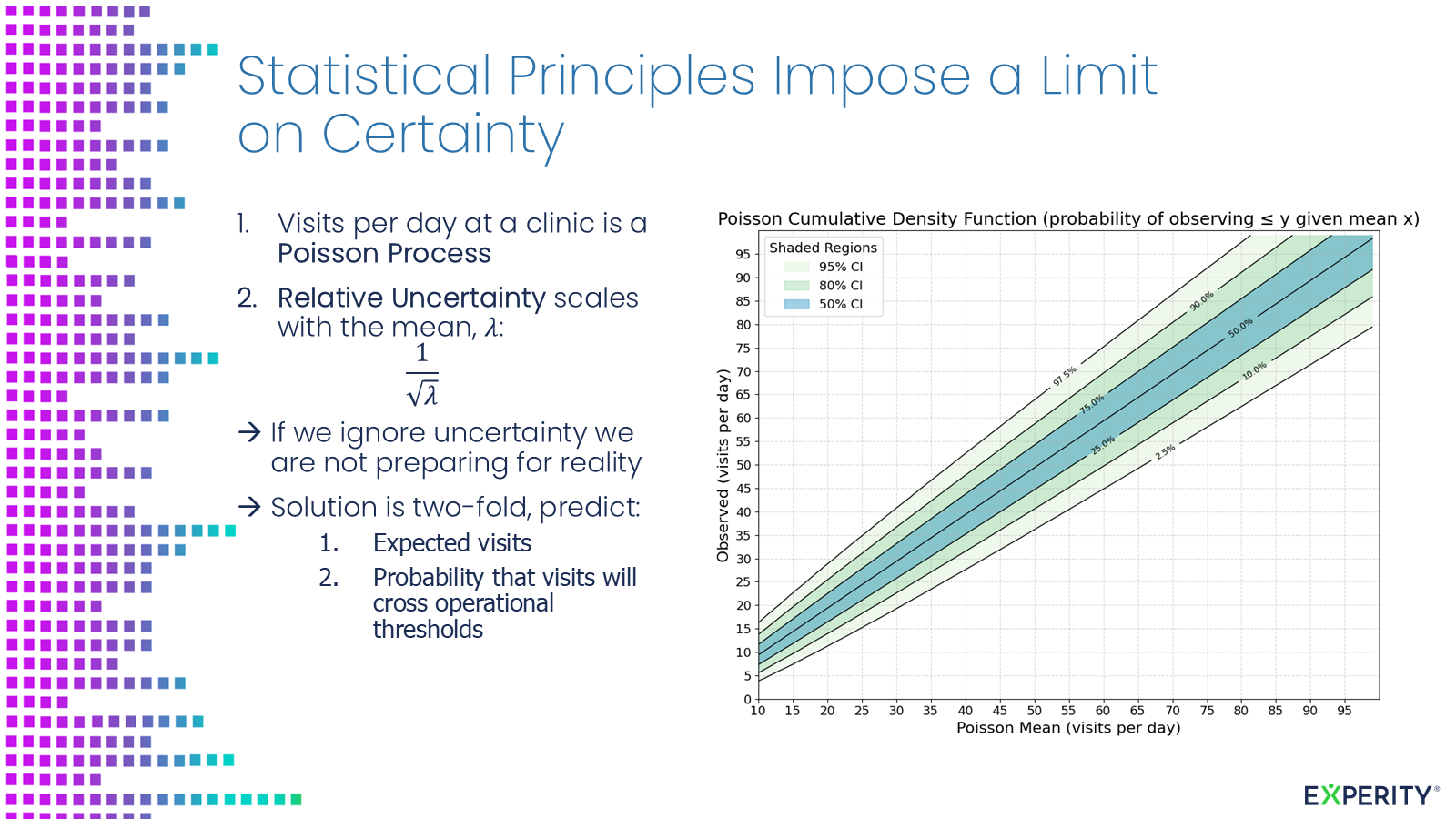
Patient visits are counts generated by individual arrivals, not a smooth signal. Even if a clinic’s expected demand were known perfectly, the observed count would still vary.

A useful starting point is a Poisson observation model:

\[Y_t \mid \lambda_t \sim \operatorname{Poisson}(\lambda_t)\]

Here, \(\lambda_t\) is expected demand after accounting for information such as clinic, day of week, seasonality, and disease activity. Under this model:

\[E(Y_t \mid \lambda_t) = Var(Y_t \mid \lambda_t) = \lambda_t\]

The standard deviation is \(\sqrt{\lambda_t}\). If expected demand is 25 visits, normal day-to-day variation is still measured in several patients. Predicting exactly 25 is therefore not the standard by which the forecast should succeed.

Poisson is a baseline, not a conclusion. Real clinic counts can have more variation than Poisson allows because of weather, outbreaks, closures, local events, or unmeasured differences among days. That overdispersion has to be tested; when it persists, a negative-binomial or another count distribution may be more credible.

The point is not that patient volume is always Poisson. It is that the observation process has variance even after the expected level has been modeled.

Separating two sources of uncertainty

The system had to represent two different unknowns.

First, expected demand is uncertain. Historical visits, diagnoses, epidemiological signals, calendar effects, and staffing patterns help estimate \(\lambda_t\), but the future drivers and the fitted model are imperfect.

Second, realized arrivals are uncertain. Even for a fixed \(\lambda_t\), the count that walks through the door varies.

The first includes uncertainty from the fitted model and from future predictors; the second is conditional count variation. A more complex model may improve the estimate of expected demand, but it cannot remove the randomness of individual arrivals.

I combined the forecast distribution with the count observation process to produce a distribution of future observed demand. The output was a range of plausible volumes—not a line presented with false precision.

Forecasting the decision

Clinic staffing changes in steps. A planned team supports demand up to some operational capacity, \(c\); beyond that level, another provider or support role may be needed. The relevant forecast is:

\[P(Y_{t+h} > c \mid \mathcal{D})\]

where \(\mathcal{D}\) represents the information available when the forecast is issued. This probability connects directly to a policy:

Add coverage when the probability of exceeding capacity is high enough.

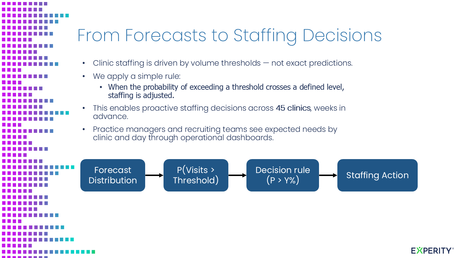
“High enough” is not purely a statistical choice. It reflects the relative consequences of excess staffing and insufficient capacity: labor cost on one side; waits, staff strain, walkouts, and patient experience on the other. The appropriate threshold can differ by clinic, role, and operating context.

In formal terms, the action should minimize expected loss:

\[a^* = \underset{a}{\operatorname{argmin}}\; E[L(a,Y_{t+h}) \mid \mathcal{D}]\]

In practical terms, this means model quality cannot be separated from the decision it supports. Reducing mean absolute error by a fraction of a visit is less useful if the model remains overconfident on high-demand days.

Testing whether the probabilities can be trusted

Once a forecast drives a threshold decision, point accuracy is no longer sufficient. A model can have a respectable average error and still assign poor probabilities.

Evaluation should reproduce the real planning process with rolling, out-of-time tests at the same forecast horizons used by operations. The important checks include:

• Calibration: when the model reports an 80% interval, does it contain roughly 80% of outcomes?
• Upper-tail performance: does it assign enough probability to unusually busy days?
• Stability: does calibration hold across clinics, seasons, and volume levels?
• Data realism: was every input actually available when the historical forecast would have been issued?

These checks are not secondary diagnostics. If an operational team acts on a stated probability, calibration is part of the product.

What this changed

The production chain became multi-source data → forecast distribution → capacity risk → staffing decision. Practice managers and recruiting could consider needs by clinic and day weeks ahead across 45 locations. Volume stopped being only a retrospective dashboard metric and became a forward-looking staffing input; thresholds could differ by clinic and role to reflect asymmetric costs of over- and under-staffing. Calibration and upper-tail checks became product requirements because teams were expected to act on stated probabilities.

The model did not eliminate uncertainty. It expressed that uncertainty in the same terms as the decision and delivered it early enough to act.

This modeling work depended on the enterprise platform beneath it: governed visit histories, consistent clinic definitions, reliable external signals, scheduled pipelines, and a production path for model outputs. I describe that broader system in From Insight to Action: Building an Enterprise Data Platform for Urgent Care.

The central lesson is simple: prediction is an intermediate product. The objective is a better decision under uncertainty.